Applications / Flow imaging
Volumetric PIV with one camera
PET-PIV is a monocular 3D PIV method: it measures a three-dimensional, three-component velocity field through a single camera. One thin phase mask is added to an otherwise conventional PIV setup, and deep-learning reconstruction recovers the flow, including at high seeding densities.
- Status
- Demonstrated in water, at laboratory scale and under a microscope
- Benchmark
- Four-camera tomographic PIV. Velocity magnitude correlates at about 0.97 to 0.98
- Processing
- About 30× faster than the tomographic reference: 1 s per frame against 30 s
- Paper
- arXiv:2607.29163 (2026)
Why one camera
Volumetric PIV usually triangulates between several cameras, typically four to six. Each camera adds cost, most of all at high speed, and needs its own view into the flow at a different angle. All of them have to be aligned, calibrated against each other to a fraction of a pixel and kept synchronized, and the tomographic reconstruction is slow.
Encoding depth through one camera removes the triangulation. The camera side of the experiment becomes a single optical path, with no alignment, calibration or synchronization between cameras to maintain.
| Multi-camera tomographic PIV | PET-PIV | |
|---|---|---|
| Cameras | Typically four to six | One |
| Views into the flow | Several, at different angles | One |
| Between cameras | Alignment, sub-pixel calibration, synchronization | Nothing to align or synchronize |
| Added optics | None | One phase mask at the lens aperture |
| Processing | About 30 s per frame in the published comparison | About 1 s per frame, or 30× faster |
| Still required | Illumination, seeding, optical access | The same |
What you add to an existing setup
The only hardware change is one thin phase mask, placed at the iris of the camera lens or, in a microscope, beneath the objective. We design a mask for your optical configuration and wavelength, and fabricate it. Standard commercial lenses, cameras and suitable PIV lasers can otherwise be used.
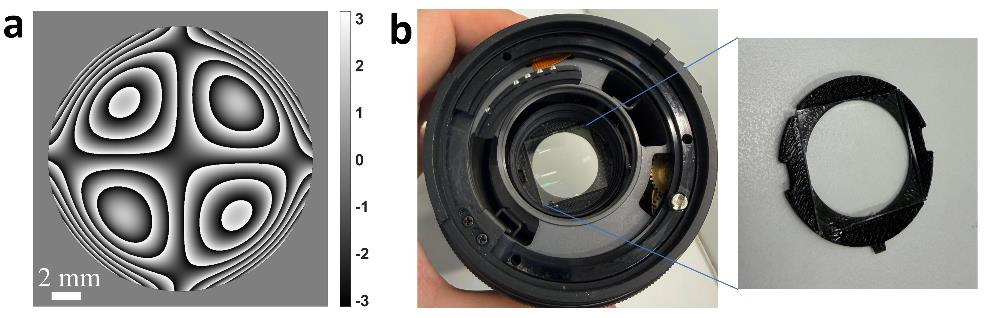
The camera’s depth response is then calibrated in place, from images of sparsely seeded flow and the known thickness of the illuminated volume.
From images to velocity fields
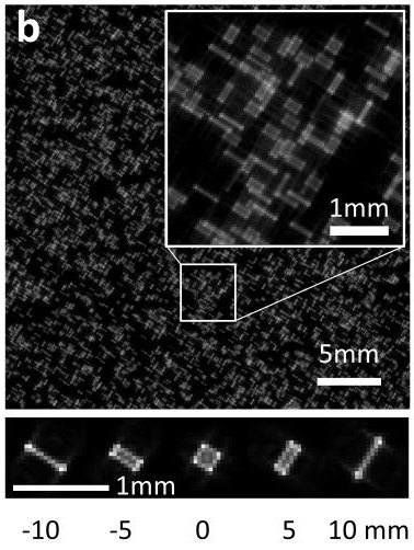
With the mask in place, each particle reaches the sensor as a shape that depends on its depth (Fig. 3). These shapes are larger than in-focus particle images and overlap as the seeding gets denser, which is why single-camera 3D methods have generally been limited to sparse seeding.
PET-PIV resolves the overlap computationally, with deep-learning code developed in Prof. Shechtman’s group. It works in two modes.
Tracking mode
Locates every particle in three dimensions, links the positions into trajectories and interpolates them onto a grid. It returns particle positions, tracks and the velocity field. Its network is trained on synthetic images generated from the calibrated model of the optics, so it needs no multi-camera reference.
Tested at 0.05 to 0.2 particles per mm³
Field mode
For seeding too dense to separate individual particles. A second network maps five consecutive frames directly to the three-dimensional velocity field. It is currently trained with reference data from tomographic PIV.
Validated at about 0.4 particles per mm³
This is research software today, not a packaged product. Its processing is already about 30× faster than the tomographic reference, and we are heading toward real-time monocular PIV.
What has been shown
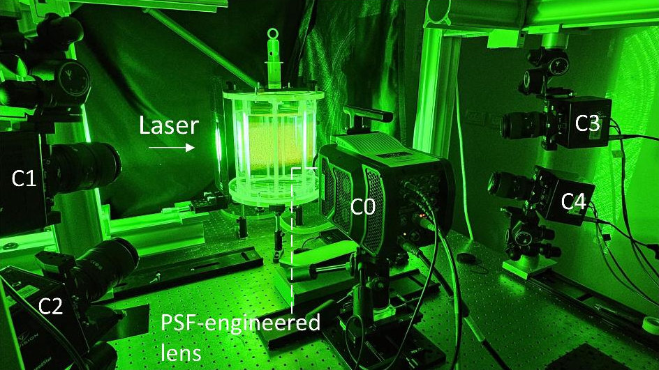
The published experiments measured swirling and jet flows in a water tank seeded with fluorescent tracer particles, at Reynolds numbers in the low thousands. A four-camera tomographic PIV system recorded the same flows at the same time and served as the reference (Fig. 4).
| Flow | Mode | Seeding density | Correlation with the reference |
|---|---|---|---|
| Swirl | Tracking | 0.1 particles per mm³ | About 0.98 |
| Jet, Re 3000 | Tracking | 0.1 particles per mm³ | About 0.97 |
| Jet, Re 2000 | Field | About 0.4 particles per mm³ | About 0.98 |
Correlation coefficient of velocity magnitude between PET-PIV and the four-camera reference, averaged over 100 frames for the swirl and 300 frames for each jet. The reference was processed with Shake-The-Box for the tracking-mode comparisons and with tomographic PIV for the field-mode comparison. Values for each velocity component are in the paper’s supplement.
Under a microscope, the tracking mode measured steady and unsteady flows in microfluidic channels 20 to 100 µm deep, through 20× and 40× objectives.
Four of these measurements can be played in Fig. 5: the frames the single camera recorded, and what was measured from them.
Swirling flow. Tracking mode, 0.1 particles per mm³.
Camera frames
Velocity field: reference, PET-PIV, difference
Jet at Re 3000. Tracking mode, 0.1 particles per mm³.
Camera frames
Velocity field: reference, PET-PIV, difference
Jet at Re 2000. Field mode, about 0.4 particles per mm³, where particle images overlap too heavily to be located one by one.
Camera frames
Velocity field: reference, PET-PIV, difference
Microfluidic channel whose depth steps from 40 to 100 µm, through a 20× objective. Tracking mode.
Camera frames
Particle trajectories, colored by speed
All twelve supplementary videos are on Zenodo, and the paper is on arXiv.
What it needs
- Like any PIV measurement, it needs illumination, seeding and optical access to the measurement volume.
- Demonstrations so far are in water, with fluorescent tracer particles. Measurements in air have not been shown yet.
- Each optical configuration is calibrated in place before measuring.
- The field mode is currently trained with reference data from tomographic PIV. Training on simulated data is the planned way to remove that step. The tracking mode does not need it.
- We assess the measurement volume and acquisition conditions for each application.
How far it scales
The measurement volume is set by the optics, not by the method. The same depth encoding has been demonstrated from microscope scale to ranging at 5 km, and we expect flow measurement to be possible at scales of a kilometer and more. Seeding and reflections at those scales are a separate question.
Where it helps
PIV is used in wind tunnels, on propulsion systems and turbines, in microfluidics and in oceanic and atmospheric research. A single-camera architecture matters most where adding cameras is the hard part.
- Limited optical access: one window or one viewing direction, as in turbomachinery or endoscopic configurations.
- Test facilities where setup and calibration time is expensive, such as towing tanks and water tunnels.
- Microfluidics, through a single microscope objective.
- Existing planar PIV systems that need the third dimension with a minor modification.
Further out, one camera with fast decoding points from laboratory measurement toward monitoring the flow in running equipment: turbines, engines, combustion, cooling, pumps and compressors. That is the direction of development, not a present capability.
Working with us
We are looking for a small number of design partners for focused, funded first projects.
The first step is a short, non-confidential call. We present the technology and results, and you tell us which measurement constraints matter most in practice.